Beverly Hills Observatory

Astronomy from Beverly Hills, MD 21214!

  • Home
  • About
  • Contact
post

Orbital Period of OV Boötis

2017-07-11 By SleepIsWrong Leave a Comment

For most of the month of June I gathered photometric data for the star OV Boötis (OV Boo), an eclipsing cataclysmic variable star with a very short orbital period.  The data were acquired using the #2 16-inch with an SBIG ST8xme camera and clear filter.   The images were calibrated using BHO_ImageCalibration, and reduced using the PPX photometry program.  With the exception of the first night of observing, the exposure time for each image was 50 seconds.  Peranso period-search software was used to determine an orbital period of 3996.7 ± 1.4 seconds.

OV Boötis

Like all cataclysmic variable (CV) stars, OV Boo is a double star system in which a collapsed (white dwarf) star is siphoning material from the outer atmosphere of it’s companion star, a low-mass red dwarf that is over filling it’s Roche lobe.  There are, however,  some unique features to this star.  First of all, its orbital period is shorter than any other hydrogen-rich CV.  There are reasonably well understood reasons why the orbital period of a “normal” CV cannot be less than about 78 minutes.  Observations back up that limit; the only CVs with shorter periods are helium-rich stars.  That is, until OV Boo was discoverd.  OV Boo’s orbital period is 66.6 minutes, a full 12-minutes shorter than is though possible.  It is also the CV with the fastest proper motion.  Finally, spectra of the red dwarf star show it to be “metal” poor.  These last two points indicate that it is likely a population-II object, the only one among the 3000 or so known CVs.

One of the consequences of being a population-II (older, early generation) star is that their atmospheres lack the quantity of “metals” (elements heavier than Helium) found in population-I (younger, more recent generation) stars.  As a result, the atmospheres of population-II stars have much lower opacity.  You can think of opacity in this sense as resistance to energy escaping.   Because the atmospheres of population-II stars are more transparent they tend not to “bloat up” as much as their younger cousins and so tend to be a bit smaller for a given mass.  There is a strong correlation between the orbital period of a CV and the mean density of the secondary star such that:

P \varpropto 1/\sqrt{\rho}

where “P” is the orbital period and \rho is the secondary star’s mean density.  So we can understand why OV Boo has such a short orbital period; its secondary is smaller, thus more dense, than the population-I stars that typically are found as secondaries in CVs.

OV Boo has been the subject of a number of investigations which indicated it was similar in many ways to WZ Sge, another short orbital period CV (82 min) that has a very low mass transfer rate and only outbursts very infrequently.  In fact, in March of this year, OV Boo was observed in outburst for the very first time.  Subsequent observations by the Center for Backyard Astrophysics (CBA) detected what are called “superhumps” in its early outburst phase, confirming its membership in the WZ Sge class.

Better Late than Never?

As often happens, I was not able to participate in the CBA campaign to monitor OV Boo’s outburst, due to a combination of lousy weather and being very busy running and, ultimately, selling my business (Orion Studios).  Still, I wanted to see if I could nail down the orbital period.  Doing so would require the deepest photometry I’ve yet attempted from BHO as the eclipses take OV Boo’s brightness to as low as 19th magnitude.  That’s a tall order for a small telescope anywhere, let alone from the middle of a major city with its god-awful light pollution.  The challenge was made all the more difficult because the eclipses themselves are very fast.  That meant I could not take long exposures which might improve the signal-to-noise ratio of the resulting photometry.  Instead, I had to stick to shorter exposures which limited the precision of my measurements to around \pm 0.05 magnitudes.

Observations of OV Boo - June 2017

DateNumber of ImagesNumber of Eclipses
2017 June 01/021003
2017 June 02/031953
2017 June 03/042293
2017 June 08/092373
2017 June 09/102163
2017 June 24/251743
2017 June 25/262464
2017 June 27/282665

All of the exposures were 50 seconds in duration, except for the first night, where the images were 200 seconds in duration.  After that first night I decided to try increasing the sampling cadence as the eclipses were short.

Reductions and Analysis

The images were calibrated using a home-brewed python script called BHO_ImageCalibrate.  The script handles all of the usual steps of bias-subtraction, dark-image scaling and subtracting, and flat-fielding.  The photometry was performed using PPX, a program written in the IDL language.  PPX finds all of the stars in each image and performs matching of stars from one image to the next.  PPX then performs variance-weighted optimal-extraction photometry for the comparison stars and the variable star.  I used DPlot to produce the chart (shown below) illustrating the photometric results for the night of June 27/28, 2017.

As can be seen in the table of observations, I managed to catch a total of 27 eclipses.  The next step was to correct all of the observation times to heliocentric time – the time an observer on the sun would observe a given phenomenon.   The heliocentric correction removes the changing arrival time of photons due to the earth’s movement around the sun.  In the most extreme cases that time difference can be as much as 19 minutes.  The data were then fed to Peranso, which incorporates a number of period-finding algorithms.  Just looking at the chart, above, it’s obvious the period is a bit over 0.045 days.  I used Peranso’s implementation of the Lomb-Scargle algorithm to determine that the orbital period is 3996.7\pm 1.4 seconds.

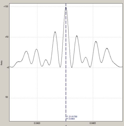
This is the periodogram created by the Lomb-Scargle function in Peranso. Essentially the higher the “significance” ( the y-axis ) the more likely it is that the period is the “correct” one. The dashed vertical line indicates the location of the periodogram’s peak – labeled as F=21.61780 cycles per day, or a period of 0.0463 days.


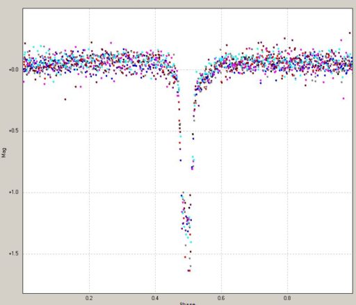
This shows all 1663 measured magnitudes, folded onto a single plot whose x-axis is scaled to one full cycle of 0.0463 days. Note that near central eclipse the data become pretty ratty. Ya – 19th mag object with short exposure times from the city!


Filed Under: Middle_1_Featured

post

Calibrating the Optec TCF-s Temperature Coefficient for a Celestron C14

2016-01-27 By SleepIsWrong Leave a Comment

About two months ago I acquired a used Optec TCF-s focuser for the telescope in the North Dome.  The focuser is designed to compensate for the changing focus position of the telescope as a function of temperature (TCF = Temperature Compensating Focuser).  It uses a temperature probe attached to the telescope tube to determine the temperature, then moves focus based on a coefficient that expresses the number of encoder steps (each resulting in 0.0022 mm movement of the focuser) per degree Celsius decline in temperature.  According to Optec’s documentation, the coefficient is around 80 steps per degree Celsius for a typical 8-inch f/10 Schmidt-Cass telescope (like a Celestron or Meade 8-inch).  Basically, as the temperature falls the telescope shrinks, reducing the distance between primary and secondary mirror.  That results in the focus point of the telescope being pushed further out (increasing “backfocus”).  Of course, I’m not using an 8-inch f/10 telescope – the ‘scope in the North Dome is a 14-inch f/11, so I needed to determine the coefficient specific to my rig.

Over the course of about a month I kept the main mirror stationary and only focused using the TCF.  I would typically re-focus every couple of hours, making note of the temperature and the position of best focus.  The chart of the results is shown below.  Given these data I arrive at a value of 161 steps per degree Celsius.  One thing that is somewhat vexing is the scatter in the plot.  One possible source of the scatter would be inaccurate temperature readings, and really is my main suspect.  For one thing, the telescope uses a dew heater strip near the front corrector plate.  That likely results in the aluminum telescope tube not being the same temperature throughout.  In the next few nights I’m going to run the dew heater at a slightly lower level to see if that reduces scatter while still keeping the corrector plate clear of dew and frost.


TCF_Coefficient


Filed Under: Hardware and Software

post

The Observatory Was Nice This Year – Look What Santa Brought!

2015-12-30 By SleepIsWrong Leave a Comment

The observatory was very good this year so Santa brought it a very nice present – a new telescope for the South Dome!  Actually it isn’t all that new.  It’s a Meade Instruments 16-inch Schmidt-Cass likely from around 1994 or so.  It has some mileage on it, and the previous owner had gutted the electronics to upgrade them with Sitech controllers and encoders which seem to be the best drive and control system for these telescopes.  Actually none of that will be of much concern as I plan to “de-fork” the telescope to place it on the Astro-Physics 1200 mount in the South Dome.  Another nice addition is a three inch Optec TCF-S3 focuser, which should be more than sufficient to support the spectrograph and camera.

The Meade Instruments 16-inch telescope just after wrestling it's 300+pounds up the stairs to my study.

The Meade Instruments 16-inch telescope just after wrestling it’s 300+pounds up the stairs to my study.

It’s sort of a shame to waste the mounting as I understand it tracks really well.  The telescope’s previous owner was able to use it to track satellites across the sky keeping the object centered in the field the whole time.  But the AP1200 is actually a much better mount and is much more compact – definitely an issue.  Furthermore, because of the short fork, the camera and spectrograph would limit how far north the telescope could point as they would not pass between the forks without hitting the base.  Anything northward of about +55 or +60 degrees would be out of reach.  That’s not a whole lot of sky but there are objects in my observing programs that would no longer be available.

Once the dovetail rail (used to attach the telescope to the mount) arrives I’ll begin testing the optics.  Meade Instruments were known to deliver some clunkers, optically speaking.  I’m also already aware of other common problems with this model, including mirror flop.  That’s why I acquired the Optec focuser.  I plan to lock the mirror down to prevent it from “floating” around – which can affect pointing and image quality.  Not surprisingly it has been raining since the telescope arrived home.

Filed Under: Hardware and Software

post

Automating the LHiRes III Calibration Lamps

2015-03-15 By SleepIsWrong Leave a Comment

The recent upgrades to the LHiRes III spectrograph include an improved calibration lamp assembly that basically has three positions:

  1. Straight through (normal data acquisition)
  2. Flat Calibration Lamp
  3. Neon-Argon Wavelength Calibration Lamp

There is a multi-pin connector that allows the observer to send 12 volts to the device and to switch to any of the three positions. Normally one would just send 12 volts to the spectrograph and use the switches mounted on the side of the instrument to select the desired mode. But the multi-pin connector was designed with remote operation in mind so I decided to assemble a simple hardware and software solution that would allow me to do so over my home’s wi-fi network.

The first challenge is to get the necessary connectors and to solder a 4-coductor wire to the connectors’ tiny pins. The connectors are “tiny xlr” style occasionally employed in music gear. It was a sore test of my non-existent soldering skills!

The main piece of the system is a model B Raspberry Pi. It’s certainly a bit of overkill as the Pi is a full-blown computer running Denbian – a Unix flavor operating system. But I figure that I may also use the Pi for other automation tasks such as building a dome controller. I found a 4-relay “hat” that fits over the GPIO pins of the Pi, allowing me to switch power to four devices. I use three to select the three positions of the calibration assembly, while the fourth currently switches the power going to the AP1200 telescope mount. I bought a small plastic box and mounted the Raspberry Pi and relay board inside, and installed two connectors, one for power input and the other to send power to the LHiRes III. For about ten dollars I bought a “WiPi” adapter for the Pi which allows control over my home WiFi network. Finally, to make it all work from the warm confines of my upstairs study in the house I wrote a simple Visual Basic program that communicates with the Pi and actuates the switches. It all works great!

The Raspberry Pi board plus 4-relay “hat” installed in a small plastic box. The cable coming from the bottom of the picture is the power in – using the Shelyak-supplied power cable, while the output cable to the LHiRes can be seen at the top of the image. The blue glowing appendage seen inside the box on the left side is the WiPi module.


The first “improvement” I need to make is to mount a switch on the box to allow me to bypass the Raspberry Pi in order to use use the switches on the LHiRes to turn the lamps off and on when I’m in the observatory.


The next task is to create a small class library for the control so that I can incorporate the automation into scripts that can be run from Maxim DL, which is what I use for controlling the cameras and data acquisition.


A view of the small control used to remotely control the calibration lamps on the LHiRes. Since there were four relays I decided to use the extra one to turn the mount on and off. The spectrum is of the star Alnilam the center star in the belt of Orion


Buffy the Lab Assistant checks the work before moving the spectrograph to the telescope


Filed Under: Hardware and Software, Uncategorized

post

Testing the Wavelength Stability of the LHiRes III Spectrograph

2015-01-18 By SleepIsWrong 2 Comments


Last summer and fall I participated in the “BRITE Stars in Cygnus” campaign monitoring the radial pulsations of Deneb’s atmosphere.  This involved measuring radial velocities by determining the wavelength shifts of the Si II λλ 6347 & 6371 lines, where expected velocity differences might be 10 km/sec or less.  After measuring a number of nights’ data it appears I’ve achieved less than “stellar” results.  On most nights the standard deviation in my data was around 2 to 3 km/sec where my goal was for a precision of 1 km/sec or better.  So I began to wonder about the wavelength stability of the LHiRes III and read a couple of posts from other observers who shared the same concern.  So I decided to conduct a few tests.  This article presents the results of a couple of those tests.

Test #1:

The first test was very simple. I took a series of calibration lamp exposures over the course of about an hour. The spectrograph was on the telescope and the telescope pointed at the pole with the drive turned off. That is, the telescope was not moving. I turned on the lamp and took an image about every two minutes. I then measured the mean shift of the three Neon lines visible in the wavelength range (Ne 6532, 6598, & 6678) recorded using an ST8 camera and the 2400 lines/mm grating, resulting in a measured dispersion of about 0.11A per pixel. Using the IRAF task “reidentify” I measured the shift from the first image and created the plot shown in Figure #1.

Figure 1: The measured shifts of calibration lines from frames taken while the telescope was “parked” – standing still, and not touching the spectrograph.

Note that, except for the very beginning, the shift in positions for the Neon lines was fairly constant wrt time. I show two linear least-squares fits – one for the entire data set and one “cherry picking” the final 3000 seconds or so. Basically the only thing this should be showing is the effects of changing temperature since nothing else was moved, other than to switch on the lamp at the beginning of the test. The telescope had been parked for over a day at the time of the test. Since the test was taken in the late afternoon the temperatures were falling – around 2 degrees C over the course of the test. The cause of the rapid drop in the roughly six-minute span near the beginning of the sequence is a mystery.


Test #2

Test #1 should give an idea of “best case scenario”. The telescope was standing still and the spectrograph was not touched throughout the duration of the test. When I’m gathering actual “science” data I always take calibration images before and after each spectrum, or around every 30 minutes in cases where I have a bright target for which I take several images within that time. Using two calibration images the wavelength solutions for surrounding calibrations are interpolated over time to match the time of mid exposure of the science image. Of course that means I need to switch the lamp on, rotate the source onto the slit, take the calibration image, rotate the source back away from the slit and turn the lamp off for each calibration image, all of which involves manipulating items which are parts of the spectrograph. Furthermore, the telescope is moving from east to west causing the direction of pull due to gravity to change throughout the sequence. So a second, more “real world” test was conducted monitoring a star with a well-determined radial velocity (HD 82885 = 11 LMi) over the course of four hours comprising a total of 11 images.


The second plot shows heliocentric-corrected measurements of radial velocity using the H-alpha line in the spectrum of HD82885. In this case the standard deviation of the measurements was 1.13 km/second. Which, to be honest, I found quite surprising. I took an additional step and used the telluric correction task in ISIS to determine the precision of the wavelength solutions and found a standard deviation of 0.04 Angstroms with a mean of essentially zero. Obviously my skill at trying to “eyeball” match the telluric lines was not all that good on an individual basis, but on average they confirmed the wavelength solutions as being generally good.


So, again, I find this result very encouraging. During the sequence of spectra the star passed across the meridian. The sequence began at hour angle -2.6 hours and finished at hour angle +1.5 hours, so a little over four hours. That means the stresses due to gravity on the spectrograph and camera changed a lot throughout the sequence. Note how the slope of the measurement curve changes at meridian crossing, hinting at slightly non-linear changes wrt hour angle likely due to gravity.


The one thing that is quite puzzling, however, was that my mean radial velocity determined from the experiment was 17.5 +/- 1.1 km/second – the published radial velocity for HD82885 is 14.4km/second. So my measurement is about 3.1 km/sec (or nearly three sigma) from the star’s known radial velocity. On the other hand, using Telluric lines in ISIS seems to agree with my wavelength solutions since, on average (despite a larger scatter in the measurements) the mean difference was zero (actually about 6e-10 Angstroms – WAY down in the noise). I have no idea what the source of the 3.1 km/sec difference is. I used 6562.801 Angstroms for the in-air wavelength of H-alpha. And I’m almost certain I measured the correct star; 11 LMi is the only 5th magnitudes star in the near vicinity and the spectra I measured match those of the star’s published G8+V spectral type.

Figure 2: Radial velocity measurements based on a four-hour sequence of 11 spectra of HD82885, a star whose radial velocity is well-known to be 14.4 km/sec. My result of 17.5 km/sec, while consistent, is consistently off by an average of 3.1 km/sec.


As a final check I used the cross-correlation task in ISIS to measure the differences of each reduced spectrum against the first spectrum. In each case ISIS reported shifts wrt the first spectrum which agreed with those I’d determined by simply measuring the position (in IRAF) of the H-alpha line.


So, in summation – it appears the LHiRes, at least for the duration of these two experiments, behaved rather well. Really surprisingly well given my previous attempts at radial velocity measurements. However, despite the standard deviation of the 11 measurements I made being just slightly above 1 km/sec, the mean ws off by 3.1 km/sec

The Sequel:

Harboring a bit of doubt about the result, above, I re-ran the experiment on the night of 2015 January 15/16. This time I only acquired 7 spectra of HD82885, but they were all a bit better S/N as I took 1800 second exposures each, as opposed to 1200 seconds for the December data. The results were even, to me, simultaneously more astonishing and perplexing. I basically found the same radial velocity, this time Vr=17.18 +/- 0.39 km/sec. So while the mean radial velocity was not significantly different the standard deviation of the measurements was even better. Note that, in both cases, I had to actually hold the knob that rotates the Neon lamp onto the slit each time. It was fairly cold outside (around -7C) and the wires inside the spectrograph that attach to the Neon source were stiff and would, if I did not hold it, cause the Neon lamp to spring back out of the light path. So I actually had to hold on to the knob during the short (2-second) calibration exposures. Figure 3 illustrates the result.

Figure 3: Result from re-running the radial velocity test illustrated in Figure 2. Within the error margins the mean radial velocity found here is the same as for the previous test, but the standard deviation is even better.


Conclusions:

Based on these two experiments (hardly an exhaustive sample):

  1. I seem to have a systematic offset of around 0.065 Angstroms, resulting in a roughly +3 km/sec error (or a bit more than 1/2 a pixel for my setup) in the region of 6600 Angstroms.  I’m not sure if that arises from instrumental issues or from my method of measuring the H-alpha absorption line in my spectra.  All measurements were done using the IRAF “splot” task.  For H-alpha in air I used 6562.801 Angstroms, and c=299700 km/sec
  2. The LHiRes III can be used to measure radial velocities within +/- 1 km/sec, perhaps better, at ~6500 Angstroms.
  3. While there is some movement within the instrument those movements seem largely linear over time. Note this says nothing about the source of such movements just that they can be calibrated out by using surrounding calibration exposures and interpolating the wavelength solutions to the central time of exposure of the “science” image.
  4. The only explanation I have for the much higher standard errors I found in my Deneb measurements is that I was adjusting the grating twice each night in order to capture both H-alpha and Si II λλ 6347 & 6371 lines. My current working theory is that after moving the grating micrometer it takes some time for things to settle.


Filed Under: Hardware and Software

post

ASAS-SN14mv

2015-01-03 By SleepIsWrong Leave a Comment

Guess What I Was Doing New Year’s Eve?

It was clear here on New Year’s Eve and I decided to try something a bit different.  I installed the 150 line/mm grating in the spectrograph and tried to acquire a spectrum of a newly-discovered transient object called ASAS-SN14mv.  It appears to be a dwarf nova in outburst and since I gather lots of photometric data on cataclysmic variables, and dwarf novae in particular, it made sense to try.  The object was at about 12th magnitude so I knew it would be a challenge.  Figure #1 is the resulting spectrum from the combination of three 1800-second exposures.

Figure #1:

Figure #1: 5400 second exposure of ASAS-SN14mv. The two most prominent lines visible are of ionized Magnesium (4481 – left side) and molecular oxygen (O2) from the earth’s atmosphere at 6867- 6944 Angstroms.


Note the absence of hydrogen lines.  In fact, when compared to the spectrum of an A0V star (like Vega) the spectrum is fairly similar except for this absence.  Outbursts of dwarf novae originate in the accretion disk surrounding the white dwarf star in a very close double-star system.  During the early stages of the outburst the disk reaches a temperature similar to the photosphere of a star like Vega, around 10,000 K, so not surprising that it’s continuum shape would mimic that of Vega.  Prior to outburst (in quiescence) these objects typically have obvious emission lines of hydrogen and helium.  But the light from the outburst overwhelms the brightness of the emission lines and, conversely, usually show broad lines of hydrogen absorption, sometimes with small emission peaks in their centers.  At the time these data were acquired ASAS-SN14mv was likely very close to it’s maximum brightness (around 12th magnitude).  The spectrum shows hints at a number of lines other than the two mentioned in the caption, but being a fairly novice spectroscopist I’m hesitant to say for sure what they are.  But comparing to A-type stars (objects with similar surface temperatures) I could guess that Fe II λ4926 is present,  as well as badly subtracted sodium night sky lines at λ5683-5688, mercury at λ5460, and another sodium doublet at λ5890-5896.  In fact the biggest challenge with the extraction of these spectra from the 2-d images was to get accurate subtractions of night sky lines.  Figure 2 shows what one of the spectra looked like before being extracted.  Figure 3 is a spectrum of the night skies here.  Pretty dreadful!


Figure #2:  This is one of the three 1800-second exposures of ASAS-SN14mv.  The star's spectrum is the bright horizontal line through the middle of the image - the bright vertical features are almost all from light pollution, mostly from high-pressure sodium and mercury outdoor lighting.

Figure #2: This is one of the three 1800-second exposures of ASAS-SN14mv. The star’s spectrum is the bright horizontal line through the middle of the image – the bright vertical features are almost all from light pollution, mostly from high-pressure sodium and mercury outdoor lighting.


Figure #3:  Prominent night sky lines visible from BHO.  All except the Oxygen line at 6300 are light pollution!

Figure #3: Prominent night sky lines visible from BHO. All except the Oxygen line at 6300 are light pollution!


The fact is that some of these lines might actually be useful for wavelength calibration since my only reference lamp, at present is Neon – and there are no bright lines blueward of about 5400 Angstroms. Note that the values in the Figure 3 annotations are based on a similar plot that appears on Christian Buil’s site HERE. Christian’s site is a wealth of information for anyone interested in the topic of astronomical spectroscopy and is very highly recommended!  Clearly he’s dealing with the same bright sky problems that I do and achieves great results!

Filed Under: Results

post

Total Lunar Eclipse of October 8, 2014

2014-10-09 By SleepIsWrong Leave a Comment

I had to be at the studio early the morning of the eclipse, so these were taken from a location near the studio (on Gable street) which had a pretty good western horizon – at least for an industrial area lit up like a maximum security prison yard.  The pictures were taken with a Nikon D5100, with a 300mm telephoto.  The ISO changed depending on the light level, from ISO100 to 4000.

Early in the umbral phases - this was taken very near "second contact".

Early in the umbral phases – this was taken very near “second contact”.

A little past half way towards total - I took this one over-exposing the sunlit part of the moon in order to show the red hue of the eclipsed portion.

A little past half way towards total – I took this one over-exposing the sunlit part of the moon in order to show the red hue of the eclipsed portion.

This is just a few minutes before the beginning of totality.

This is just a few minutes before the beginning of totality.

Totally eclipsed!  The sky was already beginning to get brighter as sunrise was only about 45 minutes before sunrise.

Totally eclipsed! The sky was already beginning to get brighter as sunrise was only about 45 minutes before sunrise.

Blood Red Moon at Sunrise!  There was a tree just west of where I was set up - the brightening blue sky and red moon made a nice contrast!

Blood Red Moon at Sunrise! There was a tree just west of where I was set up – the brightening blue sky and red moon made a nice contrast!

Filed Under: Results

post

2014_10_0405

2014-10-05 By SleepIsWrong Leave a Comment

Weather

This is the first evening of real autumn!  Today was partly cloudy and fairly warm, maybe 75F – but tonight the temperatures are rapidly dropping and it is quite windy.  The low tonight should be in the mid-upper 40s.  At the beginning of the evening the seeing was just slightly better than two arcseconds, but now (9:55pm) it is worse than 3 arcseconds.  Very clear but very unsteady air.  UPDATE – around 10:00pm the seeing started to improve markedly – to around 2 arcseconds.  UPDATE – by 10:30pm the seeing had again gone to around 3 arcseconds!

Targets

Rig #1 is running another sequence of spectra for the U Montreal campaign – Deneb and PCyg, both at H-alpha, then Deneb at the Si lines.  Rig #2 is again shooting a sequence of images of GD552.  This may be my last night on this object as Joe Patterson is requesting data from several other targets.

Software

There have been several nights of good observing for which I’ve not kelp a log.  I’ve also been working on squashing bugs in the PPX program (previously PhotProc-X).  I found a bug in the PPX code that caused signal-to-noise to be very much under estimated.  It had to do with the way the weighting mask was being built and resulted, in fact, in the mask becoming almost a straight aperture photometry mask with softer edges.  After fixing the bug photometry of the typically fainter program objects improved markedly while the standard deviation of comparison star light curves increased somewhat.   Other software such as Maxim and Mira both show lower standard deviations in comparison-minus-check light curves, but PPX’s curves for fainter program objects is clearly “tighter”.  That is to be expected as the weighting mask is optimized for the program object and not the (in this case much brighter) comparison stars.

I also had some problems with the star matching program MATCH_STARS.  Once I had fixed the PPX bug I went back and re-reduced all of the data I had for GD552 over the past four years.  The data I’d acquired in 2011 had been taken using the ST9 camera and on a couple of the nights following meridian flip there was not much overlap between the template and the flipped images.  I re-wrote the main loop to allow the program, if it could not get a good set of matched stars, to go back and add another star and re-run the analysis.  The user can choose how many iterations are run before it gives up and returns zeros for every one of the fit coefficients.  There was also a small bug that caused the program not to properly order the triangle vertices with their corresponding opposite sides.  It wasn’t a huge problem but the program now is much more likely to find matched triangles when there are few overlapping stars.  Finally, once a good fit is found, all of the stars sent to MATCH_STARS are then fit which greatly increases the number of stars used to create the final transformation coefficients, the hope being that the transforms thus derived come from a larger overlap area than they might given just a few bright stars.  Changes in the resulting photometry, thus far, have been small to none.

LHiRes III

I’m beginning to have some suspicions regarding how stable the grating micrometer is.  For the U Montreal campaign I have to change the grating angle twice during the night.  What I think I’ve noticed is that following a change in grating angle it might take a few minutes for things to “settle” – I think I’ve seen the lines move very slightly between two comparison spectra taken only a minute apart.  This is something I can easily check – maybe tonight after the final program spectrum.


Out at 1:45 am – nice night – the first night that it’s felt like autumn!

Filed Under: Observatory Log

post

2014_09_1617

2014-09-17 By SleepIsWrong Leave a Comment

Weather:

Clearing and cool.  It looks to be an ideal night – lows around 60F, no wind.

Rig #1:

More spectra of the Si lines in Deneb’s spectrum, H-alpha for P-Cyg.  For the U Montreal BRITE campaign.  Most definitely have to get going on reducing all the data from this project.

Rig #2:

A long sequence on GD552, per request of Joe Patterson.  I did a series on this star two nights ago and got some decent data.  In fact the standard deviation in the comp star differential magnitudes was the lowest I’ve ever achieved, around 0.003 magnitudes.  Due in no small measure to having really solid guiding and not having to flip the telescope at the meridian.  At that declination I should be able to track about three hours past the meridian.  So far this year I’ve gotten two nights on this target – which Joe claims is refusing to show any orbital signal:

GD 552 = Cep 1 (no clear periodic signal yet). The latter is sort of baffling – we should be able to find that orbital signal (revealed by spectroscopy, so we know where it should be). It’s a star of enormous significance – probably the oldest CV in the sky – so anything we learn about it would be great. Davud Cejudo has been observing it from Spain; some long runs by USA observers would greatly help to set a stringent limit on periodic signals – or better yet, find one.

Out at 2:30am.


Filed Under: Uncategorized

post

2014_09_0304

2014-09-05 By SleepIsWrong Leave a Comment

Rig 1

Another set of spectra for the BRITE/UMontreal campaign on P Cyg and Deneb.  I am seriously behind in getting these data calibrated and sent.  Something for the next few days as the clear weather is supposed to go away for a while.

Rig 2

I monitored a new (for me) object tonight at the behest of one of the CBA members (Enrico).  J010742.6+484519, an eclipsing system with 2.5-magnitude eclipses.  Here’s a plot from last night’s data:

All in all everything worked pretty well – the “real” magnitude scale here would be about +13.0 from what is shown (the comparison star’s V magnitude is 13.0).  The standard deviation in the comparison star light curve (in blue) is only slightly above 0.005 magnitudes.  Sadly I had to throw out a fair number of exposures as there were some serious issues with the tracking in declination, ruining dozens of frames when the telescope would “jump” in declination, causing double images.

2014_09_0304


Declination Gear Stiction

The problem can be seen in plots from the autoguider logs.  The image, below, shows both before and after.  Basically the problem turned out to be stiction due to the declination worm being too tight against its gear.  Note that during guiding I had the declination motor making corrections in only one direction (southward).  The mount is not yet perfectly polar aligned and so drifts slowly to the north.  This is something I intentionally did for the CGE mounts but in this case it’s just me not having enough time to really get the azimuth adjustment right.  Anyway, in the top frame what you’re seeing is the slow drift of the guide star’s position as measured in each 4-second guide camera exposure.  As the object crosses the zero line the motor should (and did) engage to make the correction to return the star to its initial position on the chip.  But the gearing was so tight it would not move until a lot of “spring” tension had built up in the gearing and then would “snap” – and since it had not moved as commanded during all the previous corrections the result was a massive over correction.  Then the entire sequence would repeat.  The bottom panel shows the guiding after loosening the pressure between worm and wheel.  There is still a slight bit of the same phenomenon occurring, at a much smaller scale.  Earlier today (writing this on 4-September) I loosened the worm and gear a bit more and added a touch of lithium grease to the spur gear assembly.  In the next week or two I’ll be taking both of the motor assemblies off to clean and re-grease the main worms and gears.


Autoguider3

Filed Under: Observatory Log

Next Page »

Recent Posts

  • Orbital Period of OV Boötis
  • Calibrating the Optec TCF-s Temperature Coefficient for a Celestron C14
  • The Observatory Was Nice This Year – Look What Santa Brought!
  • Automating the LHiRes III Calibration Lamps
  • Testing the Wavelength Stability of the LHiRes III Spectrograph
  • ASAS-SN14mv
  • Total Lunar Eclipse of October 8, 2014
  • 2014_10_0405
  • 2014_09_1617
  • 2014_09_0304

Post Categories

  • Hardware and Software
  • Middle_1_Featured
  • Observatory Log
  • Results
  • Uncategorized

Archives

Site Search

You are here!

Beverly Hills Observatory > Articles by: SleepIsWrong

Organizations

  • American Assn. of Variable Star Observers
  • Center for Backyard Astrophysics
  • Society for Astronomical Sciences
  • Astro. Ring for Access to Spectroscopy
  • International Dark-Sky Assoc

Software

  • IDL
  • Mirametrics Software (MIRA)
  • Image Reduction & Analysis Facility (IRAF)
  • ISIS spectroscopy software
  • Diffraction Limited Software (Maxim DL)
  • Peranso Period Finding
  • AIP4WIN
  • MPO Canopus

Hardware

  • Astro-Physics Inc.
  • Santa Barbara Instruments Group (SBIG)
  • Shelyak Instr. LHiRes III
  • Celestron Telescopes
  • Technical Innovations Observatory Domes
  • Meade Instruments

Websites

  • Cloudy Nights Astro. Fora
  • Astromart Classifieds
  • Christian Buil’s HomePage
  • Robin Leadbetter’s HomePage
  • Kalamazoo Astronomical Society
  • Grand Rapids Amateur Astro Assn
  • Westminster (MD) Astro Soc

Copyright © 2023 by Mike Potter